As an example, we are considering data described by Volkow et al. [5]. In their study the effect of alcohol on brain uptake of 11C-acetate was examined in two groups, heavy drinkers (HD) and occasional social drinkers (OSD). PET measurements of SUV in 7 brain regions (ROIs) was performed twice in each individual, under the condition (COND) of exposure to placebo or alcohol.
Simulated data were generated based on the summary data shown in figure 4B of the paper with 15 subjects in each group. Two sources of Gaussian variance were assumed, one component (S.D. = 0.1) having the same effect on all regions of each individual, and residual variance as another component affecting all regional values independently (with same S.D.). In the paper, a strong effect of condition (higher uptake of 11C-acetate during exposure to alcohol) was described in all regions, and there was a tendency for HD to have higher brain uptake of 11C-acetate than OSD when exposed to alcohol.
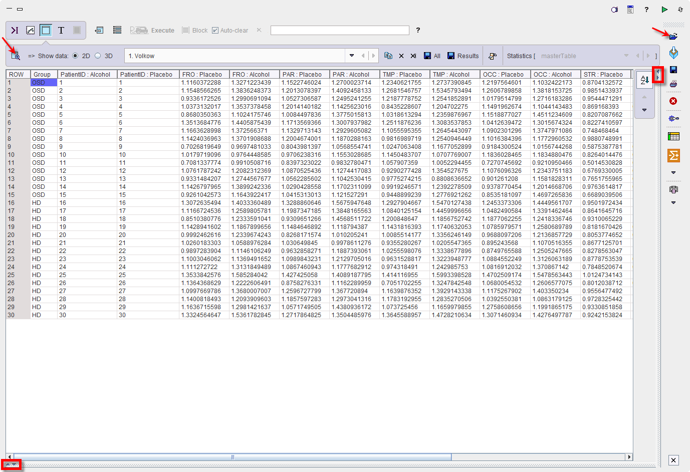
To start the analysis load the example Volkow_rmAnova.RData workspace which is available in the Pmod example database. Use the Load/Workspace Data option from the lateral task bar. It already contains the master table which forms the basis for the analysis. To visualize the master table select the Table layout icon as shown below:
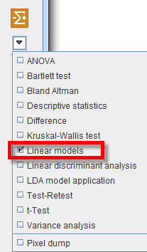
Select the Linear models entry in the scripts list as illustrated below:
The linear model interface opens. To select the Master table for the analysis use the selection arrow on the top. Correspondingly, summary of the master table content is shown in the lower part. Optionally the data to be analyzed can be restricted to a subset of the original master table by unchecking some of the boxes.
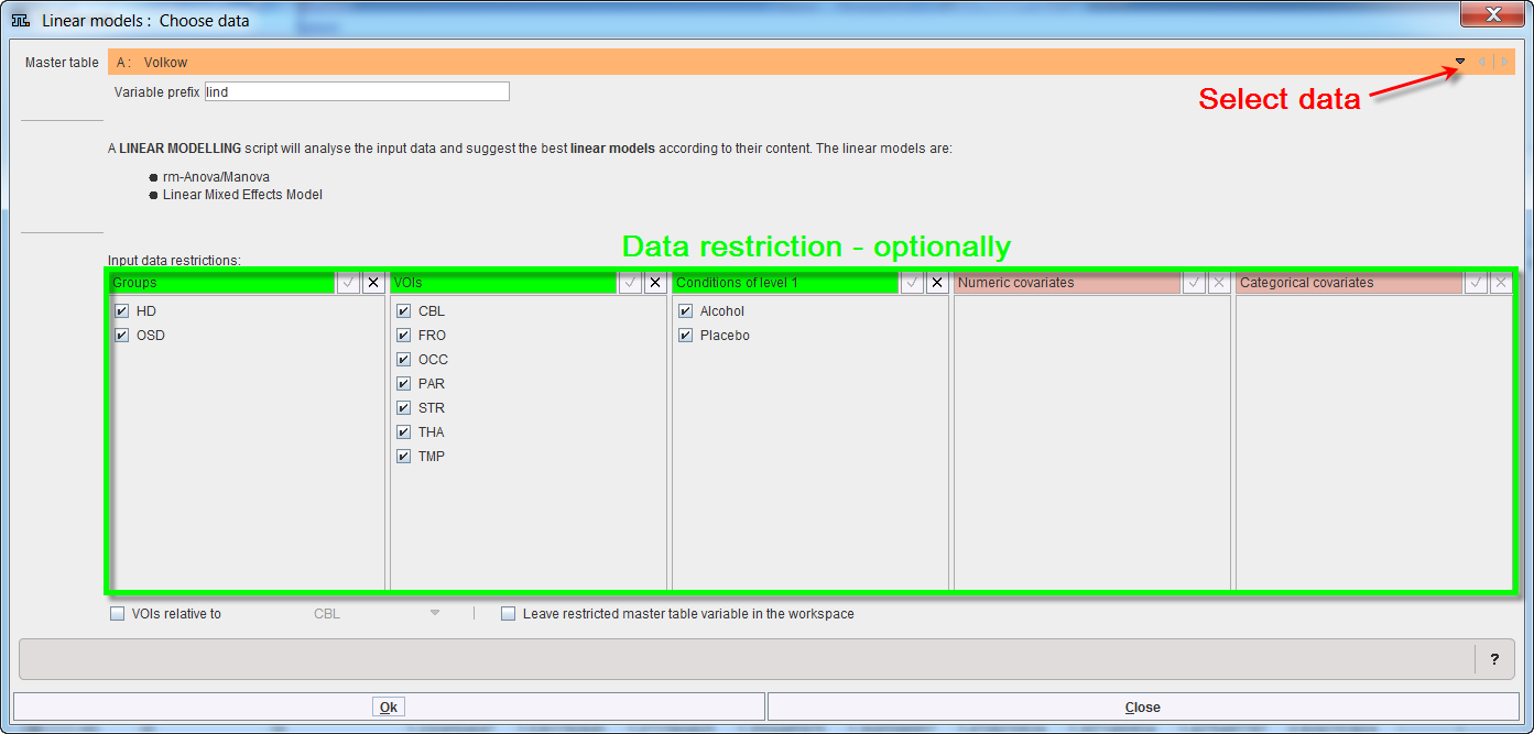
In addition, relative values can be easily obtained and used in the analysis enabling the VOIs relative to check box and selecting the reference region from the VOIs list:

The checkbox Create restricted master table variable in the workspace allows saving the new content of the restricted master table in the workspace.
Confirm the setting with the Ok button.
The program analyses the content of the "restricted" master table and provides a summary of the analysis and the suggestion for the linear model to be applied. In case the data are balanced the rm_Anova/Manova analysis is suggested by default, but the LME analysis is still available for selection.
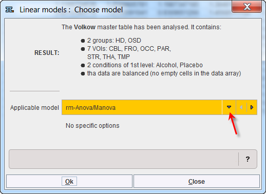
To continue the analysis activate the Ok button.
The statistical analysis is performed in the background and consists in two main step:
In the rm-Anova/MANOVA test the data columns are used as the matrix of dependent variables by the R module “lm” (R package “stats”), using a simple analysis model (columns ~ GROUP) [6]. Repeated measures ANOVA and MANOVA are then performed by the “Anova” module (package “car”) using a separate model (~ ROI + COND) for the within-subject variables [7]. Interactions between the within and between-subject variables are included by default. The result is:
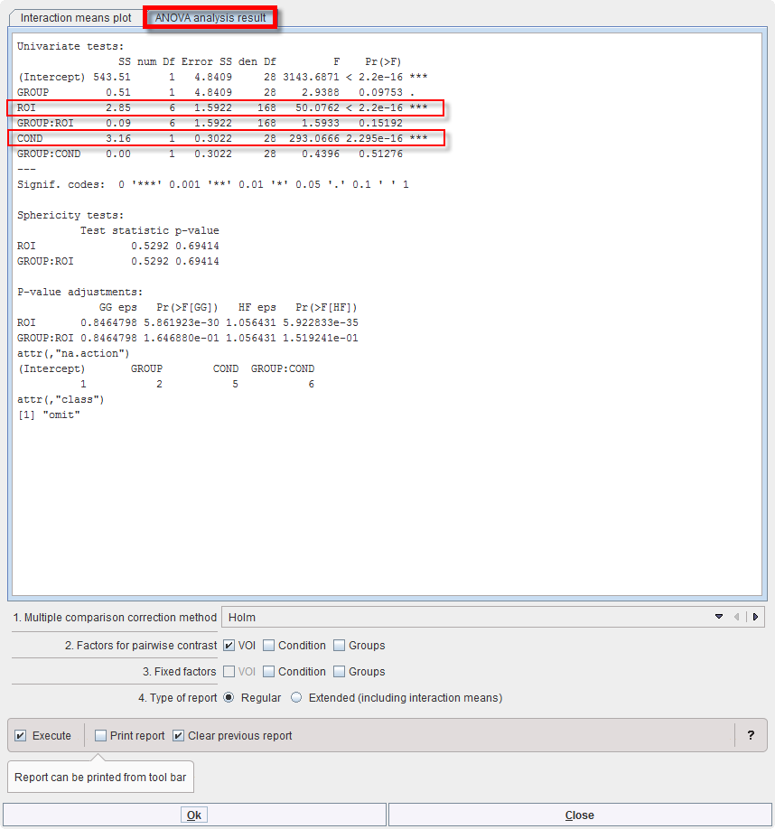
The intercept just indicates the trivial result that values are globally different from 0. Highly significant differences indicated by *** exist among ROIs (as to be expected), and between conditions (COND), which is an important experimental result. There is a trend only for a difference between groups (p=0.09). Interactions are generally non-significant. Thus, the effect of alcohol exposure on 11C-acetate uptake does not differ between groups (which is somewhat different from the results reported by the authors of the paper using actual rather than simulated data), and regional differences are similar in both groups.
Testing for sphericity does not reveal significant deviation, and accordingly the corrected P-values for ROI and the GROUP:ROI interaction do not result in a change of significance.
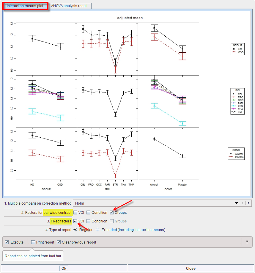
Mean values within groups and subgroups as provided by module “interactionMeans” (R package “phia”) are illustrated as a plot in the capture below. The graphic has as many rows and column as factors. The off-diagonal panels show the first-order interaction means for each pair of factors. The lack of parallelism between lines reveals how one factor changes the other one. The diagonal panels represent the marginal means of each factor.
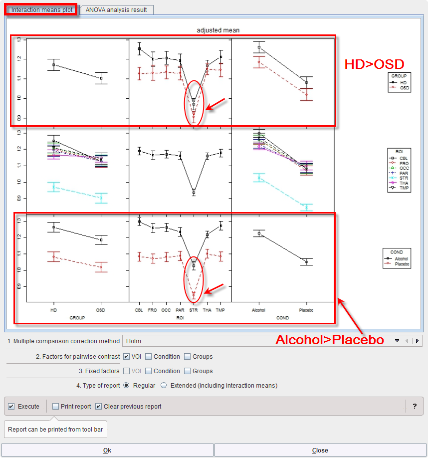
The preliminary analysis demonstrates a tendency towards higher values in group HD than OSD (top left), which is actually the case for all ROIs and conditions top row. Striatum (STR) shows much lower values than all other regions (middle panel), with minor interactions with group and condition (middle row). Values under alcohol exposure are generally higher than under placebo (bottom row).
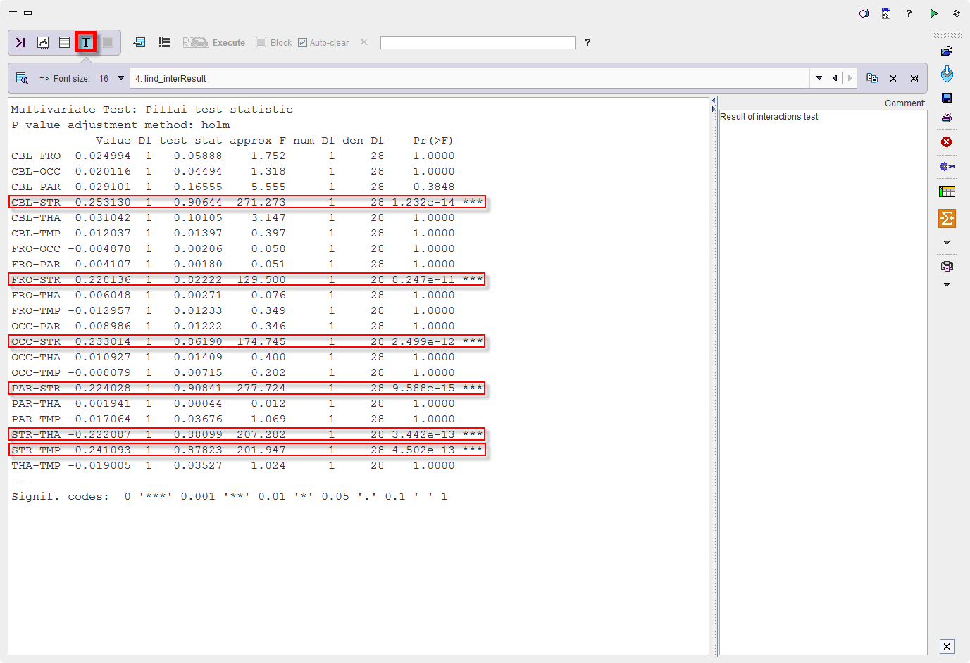
Differences between ROIs seem obvious. A pairwise analysis of their significance is provided by the module “testInteractions” from the same R package with the "Holm" method to correct for multiple comparisons and “ROI” factor for pairwise testing, while averaging over the other factors.
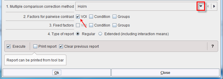
Confirm the settings for the model parameter with the Ok button. The results are displayed in the Text layout and reveal that contrasts of all regions with striatum (STR) are highly significant, but none of the other regional differences reach significance.
The results can be saved as a report activating the dedicated button  in the lateral taskbar.
Although none of the interactions was significant, one might be interested in which region showed the strongest trend towards a difference between subject groups. To achieve this, start the Linear models script again. In the Set module parameters step module “testInteractions” use VOIs as Fixed factor, and pairwise contrast of Groups as illustrated below:
The program provides the following result:
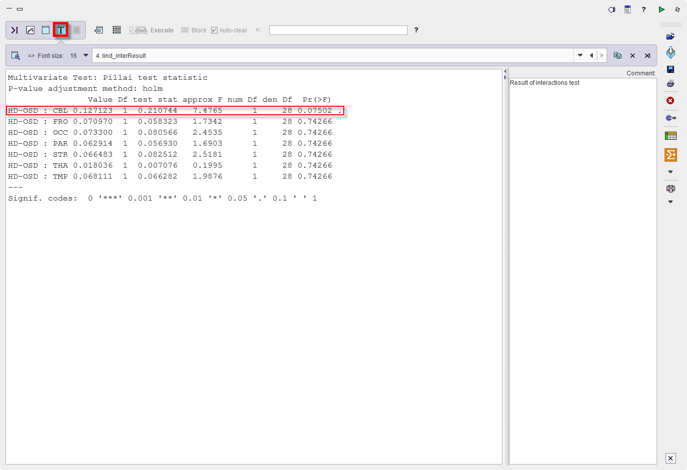
Thus, there is a trend for cerebellum (p=0.075) while all other regions are far from significance.
Overall this example demonstrates that differences between within-subject variables can be detected with high sensitivity, while differences between subject groups are more difficult to detect. In the present example, the magnitude of mean differences between groups was about half of the difference between conditions, but there was only a trend for groups, while the effect on condition was very highly significant (p<10-14). Basically this reflects the much higher power of repeat studies within subjects than comparisons between different groups of subjects, similar to the higher power of a paired t-test compared to a t-test for independent groups.